Physics for a Mathematician 02-I - The Morse-Smale-Witten Complex
I. The Mathematical Picture
The Morse-Smale-Witten Complex
At a basic level, Witten's paper uses physical reasoning to write down the so-called Morse-Smale-Witten complex. Today we will define this complex from the purely mathematical viewpoint.
I.1: Basics of Morse Theory
Suppose that $M$ is a smooth (meaning $C^{\infty}$) manifold. Suppose $f \colon M \rightarrow \mathbb{R}$ is a smooth function.
Definition: A critical point of $f$ is a point $p \in M$ such that $(df)_p = 0$.
Exercise: Suppose that $M$ is $n$-dimensional, and let $x_1,\ldots, x_n$ be local coordinates for $M$. The Hessian matrix is the matrix $$\mathrm{Hess}(f) = \left(\frac{\partial^2f}{\partial x_i \partial x_j}\right).$$ Prove that if $p \in M$ is a critical point, then the Hessian matrix defines a canonical (coordinate-independent) bilinear map $\mathrm{Hess}_p(f) \colon T_pM \times T_pM \rightarrow \mathbb{R}$ given by using the matrix of mixed partials with respect to the basis $\left(\frac{\partial}{\partial{x_1}},\ldots,\frac{\partial}{\partial{x_n}}\right)$.
Definition: A critical point $p$ of a smooth function $f \colon M \rightarrow \mathbb{R}$ is said to be non-degenerate if the Hessian matrix is a non-degenerate bilinear form. The index of $f$ at a non-degenerate critical point, denoted $\mathrm{ind}_p(f)$, is the dimension of the largest subspace of $T_pM$ on which the Hessian is a negative definite bilinear form. The function $f$ is said to be Morse if all of its critical points are non-degenerate.
One can theoretically skip the following lemma, but it is really quite useful for understanding what the Morse criterion is saying!
The Morse Lemma: If $p$ is a non-degenerate critical point of a function $f \colon M^n \rightarrow \mathbb{R}$ of index $k$, then there are local coordinates $(x_1,\ldots,x_n)$ around $p$ such that the point $p$ corresponds to the point $(0,\ldots,0)$, and $f$ takes the form $$f(x) = f(p)-\sum_{i=1}^{k}x_i^2 + \sum_{i=k+1}^{n}x_i^2.$$
Let us look at a simple example, the standard embedded $2$-sphere $S^2 \subset \mathbb{R}^3$, given by the set of points $\{(x,y,z)\mid x^2+y^2+z^2=1\}$. Consider projection to the last coordinate, $z \colon S^2 \rightarrow \mathbb{R}$. There are precisely two critical points, one at the north pole, and one out the south pole, and we will check that they are non-degenerate. Near each pole, $x$ and $y$ can be used as local coordinates, in which $z$ is expressed as $\pm \sqrt{1-x^2-y^2}$. The Hessian can be computed in these coordinates explicitly:
 |
| For $n=2$, the graphs of index $0$, $1$, and $2$ critical points. |
Let us look at a simple example, the standard embedded $2$-sphere $S^2 \subset \mathbb{R}^3$, given by the set of points $\{(x,y,z)\mid x^2+y^2+z^2=1\}$. Consider projection to the last coordinate, $z \colon S^2 \rightarrow \mathbb{R}$. There are precisely two critical points, one at the north pole, and one out the south pole, and we will check that they are non-degenerate. Near each pole, $x$ and $y$ can be used as local coordinates, in which $z$ is expressed as $\pm \sqrt{1-x^2-y^2}$. The Hessian can be computed in these coordinates explicitly:
$$\mathrm{Hess}(z) = \pm \begin{pmatrix}\frac{-x^2+y^2-1}{(1-x^2-y^2)^{3/2}} & \frac{-2xy}{(1-x^2-y^2)^{1/2}} \\ \frac{-2xy}{(1-x^2-y^2)^{1/2}} & \frac{x^2-y^2-1}{(1-x^2-y^2)^{3/2}} \end{pmatrix}$$
Here, the overall factor of $\pm 1$ corresponds to whether we are on the northern $(+1)$ or southern $(-1)$ hemisphere. Notice that the north and south poles correspond to the coordinates $(x,y) = (0,0)$, at which we compute
$$\mathrm{Hess}_p(z) = \pm \begin{pmatrix}-1 & 0 \\ 0 & -1 \end{pmatrix}.$$
We see that in either case, the critical points are non-degenerate, so $z$ is indeed a Morse function. In addition, the north pole has index two (essentially corresponding to the fact that $z$ is convex downward in two dimensions worth of directions) and the south pole has index zero (because $z$ is not convex downward in any direction).
The basic tenet of Morse theory is that all of the interesting topology (in the smooth category) of $M$ is encoded by data attached to each critical point. Let us think about why this might be the case for $S^2$ by thinking about what extra structure the function $z$ affords us. To do this, we slice the sphere up along its $z$-level sets, and try to understand what happens as we build the sphere up level by level. In particular, we want to understand what the sets $M_t = z^{-1}(-\infty,t]$ look like as $t$ increases from $-\infty$ to $+\infty$. We see that in the case of $S^2$, these level sets only change in an interesting way when $t$ passes through $\pm 1$:


- When $t < -1$, $M_t = \emptyset$.
- When $-1 < t < 1$, $M_t = \mathbb{D}^2$, a disk (up to diffeomorphism).
- When $1 < t$, $M_t = S^2$.
The values $\pm 1$ are the images of the critical points of $z$ under the map $z$, and are called critical values. The picture above suggests that the following true proposition:
Proposition: Suppose $f \colon M \rightarrow \mathbb{R}$ is a Morse function. For $t \in \mathbb{R}$, set $M_t := f^{-1}(-\infty,t]$. If $t$ is not a critical value, then $M_t$ is a (possibly empty) manifold with (possibly empty) boundary $\partial M_t = f^{-1}(t)$. Furthermore, if there are no critical values lying on the interval $[t_0,t_1]$, then $M_{t_0}$ and $M_{t_1}$ are diffeomorphic (in fact via a diffeomorphism which is the identity on its restriction to $M_{t_0-\epsilon} \subset M_{t_0}$ where $\epsilon > 0$ is chosen small enough so that there are no critical values on the interval $[t_0-\epsilon,t_0]$).
Hence, in order to study a smooth manifold $M$ from the perspective of Morse theory, it suffices to satisfactorily answer the following two questions:
Question 1: Given a smooth manifold $M$, does a Morse function $f \colon M \rightarrow \mathbb{R}$ exist? If so, if we have two Morse functions $f$ and $g$, how are they related?
Question 2: How do the submanifolds $M_t$ change when we pass through a critical value? What data encodes this change?
Both of these questions are well-understood via Morse theory. However, since our goals our a little more short-sighted, we will instead deal with a modified version of Question 2, stated as Question 2' below. This trade-off sacrifices quite a bit of mathematical motivation, but as we are after Witten's perspective after all, we shall shrug this off and call ourselves "physicists" whenever somebody asks.
Theorem: "Almost every" function from $M$ to $\mathbb{R}$ is Morse. (Here, "almost every" means that they form an open dense subset of all smooth functions in the $C^2$-topology.) Furthermore, if $f,g \colon M \rightarrow \mathbb{R}$ are two Morse functions, then there exists a family $F \colon M \times [0,1] \rightarrow \mathbb{R}$ such that:
Both of these questions are well-understood via Morse theory. However, since our goals our a little more short-sighted, we will instead deal with a modified version of Question 2, stated as Question 2' below. This trade-off sacrifices quite a bit of mathematical motivation, but as we are after Witten's perspective after all, we shall shrug this off and call ourselves "physicists" whenever somebody asks.
Question 2': How can we use Morse theory to describe nice algebraic invariants attached to $M$?
We finish this section by providing a complete answer to Question 1.
We finish this section by providing a complete answer to Question 1.
Theorem: "Almost every" function from $M$ to $\mathbb{R}$ is Morse. (Here, "almost every" means that they form an open dense subset of all smooth functions in the $C^2$-topology.) Furthermore, if $f,g \colon M \rightarrow \mathbb{R}$ are two Morse functions, then there exists a family $F \colon M \times [0,1] \rightarrow \mathbb{R}$ such that:
- $F(\cdot,0) = f$
- $F(\cdot,1) = g$
- There is a finite subset $\{t_1,\ldots,t_\ell\} \subset (0,1)$ such that $F(\cdot,t)$ is Morse when $t \neq t_i$ for all $i$.
- For each $i$, the function $F(\cdot, t_i)$ has a unique degenerate critical point $p_i$ (the other critical points all remain non-degenerate) such that there exist local coordinates around $p_i$ near $p_i$ around which $$F(x,t) = f(p_i)-\sum_{i=1}^{k}x_i^2 + \sum_{i=k+1}^{n-1}x_i^2 + x_n^3 \pm (t-t_i)x_n$$ for $t$ close to $t_i$.
We see that we either create or cancel a pair of critical points of neighboring indices $k$ and $k+1$ (depending upon whether the sign in the above local model is negative or positive, respectively) when we pass through time $t_i$. Notice that you can not simply cancel critical points of neighboring indices at random; you need to be able to put them into the position of the local model! We illustrate below a family of Morse functions on the sphere $S^2$ which passes through a degenerate critical point.
 |
| A family of Morse functions on a sphere, represented by the height function. In the middle, there is a single degenerate critical point. Before this, there were no critical points, and after this, we have created a critical point of index 1 and index 2 near each other. |
I.2: The Morse-Smale-Witten Complex
Consider a Morse function $f \colon M \rightarrow \mathbb{R}$. Suppose that $M$ is given the extra structure of a Riemannian metric $g$, meaning a positive definite symmetric $2$-tensor field. In other words, for each $x \in M$, we have an inner product $g_x$ on $T_xM$, and we require that the inner product varies in a $C^{\infty}$ manner. Recall that an inner product on a vector space $V$ determines an isomorphism $\phi \colon V \rightarrow V^*$, given by $$\phi(v)(w) = \langle v,w \rangle.$$
Definition: On a Riemannian manifold $(M,g)$, the gradient of a function $f \colon M \rightarrow \mathbb{R}$ is the vector field $\nabla_g f$ which, at the point $p \in M$, is given by $\phi_{g_p}^{-1}(df_p) \in T_p M$. In other words, $\nabla_g f$ is the vector field $g$-dual to the $1$-form $df$.
Exercise: Suppose we are in coordinates $x_1, \ldots, x_n$. Then we may write the metric as a positive-definite symmetric matrix $g_x = (g_{ij}(x))$. Then $\nabla_g f = \sum_j \left(\sum_i g_{ij}\frac{\partial f}{\partial x_i} \right) \frac{\partial}{\partial x_j}$. If we are on $\mathbb{R}^n$ with the standard metric (the standard inner product at every point in the standard coordinates of $\mathbb{R}^n$), then the gradient is the usual one you're used to from standard multivariable calculus.
So if we have a Morse function $f \colon M \rightarrow \mathbb{R}$, and we fix some metric $g$ on $M$, then we have a vector field $\nabla_g f$ on $M$. When we have such a vector field, we automatically have a differential equation that we can solve, yielding integral curves. In the case, we are looking for maps $\gamma \colon \mathbb{R} \rightarrow M$ such that $$\frac{d\gamma}{dt} = -(\nabla_g f)(\gamma(t))$$ which are called (negative) gradient flow lines since we are flowing along the negative gradient. (We will often omit the word negative, hopefully without confusion.) Just like in coordinates, also on manifolds there is an existence and uniqueness theorem for such differential equations, so if I know $\gamma(0) = p$, then I can uniquely solve to find integral curves, at least for small times. We will assume that $M$ is closed (compact without boundary) in our setting, so actually, these solutions persist for all times.
Intuitively, what these gradient flow lines are saying is the following. Suppose you have your manifold $M$, and let's think that it's a surface for simplicity, which you're holding so that gravity is pointing in some direction, and so that your given function $f \colon M \rightarrow \mathbb{R}$ is the height off the ground. Thinking about this picture as living in $\mathbb{R}^3$ gives us a standard metric, so there's a gradient flow. Suppose on your surface, there's a drop of water at a point $p$, which is free to move, but by adhesion, will stick to the surface and never fly off of it. The drop of water will then tend to follow the gradient flow lines just described!
This flow picture gives us, for each $t$, a diffeomorphism $\Phi_t^f \colon M \rightarrow M$, given by flowing along the gradient flow lines for time $t$. In other words, if $p \in M$, then $\Phi_t^f(p) := \gamma(t)$ where $\gamma$ is the unique integral curve with $\gamma(0) = p$.
Exercise: Each $\Phi_t^f$ is a diffeomorphism, and $\Phi_{t_1+t_2}^f = \Phi_{t_1}^f \circ \Phi_{t_2}^f$, so we have a group homomorphims $$\Phi_{\bullet}^{f} \colon \mathbb{R} \rightarrow \mathrm{Diff}(M).$$
Exercise: If $t > 0$, then $f(\Phi_t^f(p)) \leq f(p)$, with equality if and only if $p$ is a critical point. A similar statement holds for $t < 0$ with the reverse inequality. In other words, the integral curves always decrease the value of the function $f$. (This is intuitive from thinking about water droplets on surfaces!)
Definition: For each critical point $p$, we may consider the set of points which flow into and out of $p$. The unstable manifold $W_p^u$ of $p$ is the set of points $$W_p^u := \{q \mid \lim_{t \rightarrow -\infty} \Phi_t^f(q) = p\}.$$ Similarly, the stable manifold $W_p^s$ of $p$ is the set of points $$W_p^s := \{q \mid \lim_{t \rightarrow \infty} \Phi_t^f(q) = p\}.$$
Lemma: For each critical point $p$ of index $k$, the unstable manifold $W_p^u$ is a smooth manifold of dimension $k$, the stable manifold $W_p^s$ is a smooth manifold of codimension $k$ (i.e. dimension $n-k$), and $W_p^u$ and $W_p^s$ intersect only at the point $p$, with transverse intersection.
Proof sketch: As the stable and unstable manifolds are invariant under the gradient flow, it suffices to prove they are smooth manifolds of the correct dimension in a neighborhood of the critical point $p$. But by the Morse Lemma, we know what $f$ looks like in coordinates $p$. The tricky bit is that we can assume that the metric $g$ is constant in this neighborhood: it is approximately given by its value $g_p$ at the critical point, and you need to check that this approximation is `good enough.' Then you simply have a local computation.
We now ask the question: when are there integral curves which flow from one critical point $p_0$ to another $p_1$? This is the same as asking the question of when the intersection $$\widetilde{\mathcal{M}}(M,p_0,p_1,g,f) := W_{p_0}^u \cap W_{p_1}^s$$ is nonempty, since this is the set of points so that if you flow them backwards, you arrive at $p_0$, and if you flow them backwards, you arrive at $p_1$. Notice that $\widetilde{\mathcal{M}}$ comes with an extra translation: if $q \in \widetilde{\mathcal{M}}$, then so is $\Phi_t^f(q)$ for any $t$. Hence, we will never have that this intersection is transverse, but we can still ask that the intersections are transverse up to this translation. This condition is called the Morse-Smale condition, and we will assume it without question. For generic choices of Morse functions $f$ and metrics $g$, this condition will be satisfied. Under this condition, the dimension of $\widetilde{\mathcal{M}}$ then follows from standard transversality:
Exercise (easy if you know how to deal with transversality, difficult if not): Under the Morse-Smale condition, $\widetilde{\mathcal{M}}(M,p_0,p_1,g,f)$ is a (possibly empty) submanifold of $M$ of dimension $k_0-k_1$, where $k_i$ is the index of the critical point $p_i$. Hint: Pick a level set between $p_0$ and $p_1$. The Morse-Smale condition gives a transverse intersection on this slice.
In particular, if $k_1 > k_0$, then (under the Morse-Smale condition) there will be no gradient trajectories between the two critical points! In fact, if $k_0 = k_1$, then we expect the result will be $0$-dimensional, so just a collection of points, but by a previous exercise, the only way this will be non-empty (again under the Morse-Smale condition) is if $p_0 = p_1$. So the only interesting cases come from the case where $k_0 > k_1$. Let us focus on the case that $k_0 = k_1 + 1$. In this case, $\widetilde{\mathcal{M}}$ has dimension 1, but also, we have the translation action, which accounts for this entire dimension. In other words, we may form $\mathcal{M} := \widetilde{\mathcal{M}}/\mathbb{R}$, the moduli space of gradient trajectories, where we think of two points on the same flow line as representing the same element. This is now a $0$-dimensional manifold, or just a collection of points. In other words, in the case $k_0 = k_1 + 1$, we obtain numbers $$n(p_0,p_1) \in \mathbb{Z},$$ where we count the number of flow lines from $p_0$ to $p_1$.
WARNING: Under the rug, there are some issues of orientations, so each gradient trajectory comes with a sign. When I was an early grad student, I had this idea that they were kind of tricky, but as time has continued, I've come to think they're not so bad at all, so long as one doesn't make choices along the way. My bias is that everything should always be stated with respect to orientation lines, so that you only need to make choices when performing computations.
At this point, we can cook up an algebraic gadget as follows. For each $k \in \{0,1,\ldots,n\}$ let $$C_k = \mathbb{Z}^{S_k}$$ where $S_k$ is the set of critical points. (Non-canonically, this is just the group $\mathbb{Z}^{|S_k|}$, but I prefer to keep everything canonical.) Then we can define a map $$d_k \colon C_k \rightarrow C_{k-1}$$ by $$d_k(p) = \sum_{\mathrm{ind}(q) = k-1} n(p,q) \cdot q.$$ Hence, we have a sequence of composable maps $$0 \rightarrow C_n \xrightarrow{d_n} \cdots \xrightarrow{d_{k+1}} C_k \xrightarrow{d_k} C_{k-1} \xrightarrow{d_{k-1}} \cdots \xrightarrow{d_1} C_0 \rightarrow 0.$$
Fact: The composition $d_{k-1} \circ d_k = 0$ for each $k$. This gives us a chain complex. The details of the proof of this are surprisingly technical, but here's the main thrust of the proof. We may write $$d_{k-1} \circ d_k(p) = \sum_{\mathrm{ind}(q)=k-1} \left( \sum_{\mathrm{ind}(r)=k-1} n(p,r) \cdot n(r,q) \right) \cdot q.$$ We must prove that each coefficient $\sum_{\mathrm{ind}(r)=k-1} n(p,r) \cdot n(r,q)$ is $0$. This is the number of points, counted with signs, in the product $$\sqcup_{\mathrm{ind}(r) = k-1} \mathcal{M}(p,r) \times \mathcal{M}(r,q).$$ The key point is that this $0$-manifold is actually naturally the boundary of a compact oriented $1$-manifold with boundary, given by $\overline{\mathcal{M}(p,q)}$, where we have to say what we mean by the closure symbol. Indeed, a $1$-parameter family of trajectories from $p$ to $q$ can degenerate into a composition of flow lines from $p$ to $r$ followed by $r$ to $q$. But the boundary of an oriented $1$-manifold consists of an equal number of positive points as negative points, so indeed, we get a contribution of $0$.
This chain complex is precisely the Morse-Smale-Witten complex. Since it is indeed a chain complex, we have that the image of each $d_{k+1}$ is contained in the kernel of each $d_k$, and so we may form the Morse homology $$H_k(M,f, g) := \mathrm{ker}(d_k)/\mathrm{im}(d_{k+1}).$$
Remark: In the case that the Morse function is self-indexing, meaning that $f(p) = \mathrm{ind}(p)$ whenever $p$ is a critical point, it can be checked quite directly that the Morse homology is isomorphic to singular homology. It turns out that even in the non-self-indexing case:
Fact: The Morse homology is independent of the Morse function $f$ and the metric $g$ satisfying the Morse-Smale condition. The main way to go about proving this is to use what are called continuation maps, which essentially studies Morse trajectories on the manifold $M \times [0,1]$, with $(f_0,g_0)$ on $M \times \{0\}$ and $(f_1,g_1)$ on $M \times \{1\}$. In fact, one needs to make choices for what happens on the interior $M \times (0,1)$, but a similar argument shows that the continuation maps themselves are independent on the homology level by studying continuation maps between the continuation maps! It is much trickier to check directly that modification of the Morse function yields the same homology.
Example: Creation of a pair of critical points does not affect the Morse homology. Suppose we have a family $f_t$ of Morse functions on $M$ creating critical points, so that $f_{\epsilon}$ has two extra critical points as compared with $f_{-\epsilon}$. So long as $n > 1$, we may assume that $f_t$ is fixed in a neighborhood of the union of the submanifolds $\widetilde{\mathcal{M}(f_{-\epsilon})}$, so that the only change in the Morse-Smale-Witten complex between $f_{-\epsilon}$ and $f_{\epsilon}$ occurs with regards to gradient trajectories involving $p$ or $q$ (or both). In fact, from the local model, we have that for $f_{\epsilon}$, there is a unique trajectory from $p$ to $q$. So if $(C_*,d_*)$ is the Morse-Smale-Witten complex of $f_{-\epsilon}$, then the Morse-Smale-Witten complex of $f_{\epsilon}$ is of the form $$0 \rightarrow C_n \xrightarrow{d_n} \cdots \xrightarrow{d_{k+3}} C_{k+2} \xrightarrow{\begin{pmatrix}A \\ d_{k+2}\end{pmatrix}} \mathbb{Z} \oplus C_{k+1} \xrightarrow{\begin{pmatrix}\pm 1 & B \\ C & d_{k+1}\end{pmatrix}} \mathbb{Z} \oplus C_k \xrightarrow{\begin{pmatrix}D & d_k\end{pmatrix}} C_{k-1} \xrightarrow{d_{k-1}} \cdots \xrightarrow{d_1} C_0 \rightarrow 0$$ where the linear maps $A$, $B$, $C$, and $D$ count gradient trajectories of $f_{\epsilon}$ as follows:
Definition: On a Riemannian manifold $(M,g)$, the gradient of a function $f \colon M \rightarrow \mathbb{R}$ is the vector field $\nabla_g f$ which, at the point $p \in M$, is given by $\phi_{g_p}^{-1}(df_p) \in T_p M$. In other words, $\nabla_g f$ is the vector field $g$-dual to the $1$-form $df$.
Exercise: Suppose we are in coordinates $x_1, \ldots, x_n$. Then we may write the metric as a positive-definite symmetric matrix $g_x = (g_{ij}(x))$. Then $\nabla_g f = \sum_j \left(\sum_i g_{ij}\frac{\partial f}{\partial x_i} \right) \frac{\partial}{\partial x_j}$. If we are on $\mathbb{R}^n$ with the standard metric (the standard inner product at every point in the standard coordinates of $\mathbb{R}^n$), then the gradient is the usual one you're used to from standard multivariable calculus.
So if we have a Morse function $f \colon M \rightarrow \mathbb{R}$, and we fix some metric $g$ on $M$, then we have a vector field $\nabla_g f$ on $M$. When we have such a vector field, we automatically have a differential equation that we can solve, yielding integral curves. In the case, we are looking for maps $\gamma \colon \mathbb{R} \rightarrow M$ such that $$\frac{d\gamma}{dt} = -(\nabla_g f)(\gamma(t))$$ which are called (negative) gradient flow lines since we are flowing along the negative gradient. (We will often omit the word negative, hopefully without confusion.) Just like in coordinates, also on manifolds there is an existence and uniqueness theorem for such differential equations, so if I know $\gamma(0) = p$, then I can uniquely solve to find integral curves, at least for small times. We will assume that $M$ is closed (compact without boundary) in our setting, so actually, these solutions persist for all times.
Intuitively, what these gradient flow lines are saying is the following. Suppose you have your manifold $M$, and let's think that it's a surface for simplicity, which you're holding so that gravity is pointing in some direction, and so that your given function $f \colon M \rightarrow \mathbb{R}$ is the height off the ground. Thinking about this picture as living in $\mathbb{R}^3$ gives us a standard metric, so there's a gradient flow. Suppose on your surface, there's a drop of water at a point $p$, which is free to move, but by adhesion, will stick to the surface and never fly off of it. The drop of water will then tend to follow the gradient flow lines just described!
|
| Some gradient flow lines on the sphere $S^2$, where the Morse function is the "height" function, and we have a standard metric coming from having the picture embedded in $\mathbb{R}^3$. The critical points represent constant flow lines. Meanwhile, the trajectories "connecting" critical points never actually hit the critical points in finite time. |
This flow picture gives us, for each $t$, a diffeomorphism $\Phi_t^f \colon M \rightarrow M$, given by flowing along the gradient flow lines for time $t$. In other words, if $p \in M$, then $\Phi_t^f(p) := \gamma(t)$ where $\gamma$ is the unique integral curve with $\gamma(0) = p$.
Exercise: Each $\Phi_t^f$ is a diffeomorphism, and $\Phi_{t_1+t_2}^f = \Phi_{t_1}^f \circ \Phi_{t_2}^f$, so we have a group homomorphims $$\Phi_{\bullet}^{f} \colon \mathbb{R} \rightarrow \mathrm{Diff}(M).$$
Exercise: If $t > 0$, then $f(\Phi_t^f(p)) \leq f(p)$, with equality if and only if $p$ is a critical point. A similar statement holds for $t < 0$ with the reverse inequality. In other words, the integral curves always decrease the value of the function $f$. (This is intuitive from thinking about water droplets on surfaces!)
Definition: For each critical point $p$, we may consider the set of points which flow into and out of $p$. The unstable manifold $W_p^u$ of $p$ is the set of points $$W_p^u := \{q \mid \lim_{t \rightarrow -\infty} \Phi_t^f(q) = p\}.$$ Similarly, the stable manifold $W_p^s$ of $p$ is the set of points $$W_p^s := \{q \mid \lim_{t \rightarrow \infty} \Phi_t^f(q) = p\}.$$
Lemma: For each critical point $p$ of index $k$, the unstable manifold $W_p^u$ is a smooth manifold of dimension $k$, the stable manifold $W_p^s$ is a smooth manifold of codimension $k$ (i.e. dimension $n-k$), and $W_p^u$ and $W_p^s$ intersect only at the point $p$, with transverse intersection.
Proof sketch: As the stable and unstable manifolds are invariant under the gradient flow, it suffices to prove they are smooth manifolds of the correct dimension in a neighborhood of the critical point $p$. But by the Morse Lemma, we know what $f$ looks like in coordinates $p$. The tricky bit is that we can assume that the metric $g$ is constant in this neighborhood: it is approximately given by its value $g_p$ at the critical point, and you need to check that this approximation is `good enough.' Then you simply have a local computation.
 |
| A schematic for the stable and unstable manifolds for the (negative) gradient flow near a critical point. The particular example shown is an index $1$ critical point on a $2$-dimensional manifold in local coordinates (with the standard metric and with Morse function $f(x,y) = x^2-y^2$. More generally, one should imagine that $W_p^u$ has dimension given by the index, and $W_p^s$ has codimension given by the index. |
We now ask the question: when are there integral curves which flow from one critical point $p_0$ to another $p_1$? This is the same as asking the question of when the intersection $$\widetilde{\mathcal{M}}(M,p_0,p_1,g,f) := W_{p_0}^u \cap W_{p_1}^s$$ is nonempty, since this is the set of points so that if you flow them backwards, you arrive at $p_0$, and if you flow them backwards, you arrive at $p_1$. Notice that $\widetilde{\mathcal{M}}$ comes with an extra translation: if $q \in \widetilde{\mathcal{M}}$, then so is $\Phi_t^f(q)$ for any $t$. Hence, we will never have that this intersection is transverse, but we can still ask that the intersections are transverse up to this translation. This condition is called the Morse-Smale condition, and we will assume it without question. For generic choices of Morse functions $f$ and metrics $g$, this condition will be satisfied. Under this condition, the dimension of $\widetilde{\mathcal{M}}$ then follows from standard transversality:
Exercise (easy if you know how to deal with transversality, difficult if not): Under the Morse-Smale condition, $\widetilde{\mathcal{M}}(M,p_0,p_1,g,f)$ is a (possibly empty) submanifold of $M$ of dimension $k_0-k_1$, where $k_i$ is the index of the critical point $p_i$. Hint: Pick a level set between $p_0$ and $p_1$. The Morse-Smale condition gives a transverse intersection on this slice.
In particular, if $k_1 > k_0$, then (under the Morse-Smale condition) there will be no gradient trajectories between the two critical points! In fact, if $k_0 = k_1$, then we expect the result will be $0$-dimensional, so just a collection of points, but by a previous exercise, the only way this will be non-empty (again under the Morse-Smale condition) is if $p_0 = p_1$. So the only interesting cases come from the case where $k_0 > k_1$. Let us focus on the case that $k_0 = k_1 + 1$. In this case, $\widetilde{\mathcal{M}}$ has dimension 1, but also, we have the translation action, which accounts for this entire dimension. In other words, we may form $\mathcal{M} := \widetilde{\mathcal{M}}/\mathbb{R}$, the moduli space of gradient trajectories, where we think of two points on the same flow line as representing the same element. This is now a $0$-dimensional manifold, or just a collection of points. In other words, in the case $k_0 = k_1 + 1$, we obtain numbers $$n(p_0,p_1) \in \mathbb{Z},$$ where we count the number of flow lines from $p_0$ to $p_1$.
WARNING: Under the rug, there are some issues of orientations, so each gradient trajectory comes with a sign. When I was an early grad student, I had this idea that they were kind of tricky, but as time has continued, I've come to think they're not so bad at all, so long as one doesn't make choices along the way. My bias is that everything should always be stated with respect to orientation lines, so that you only need to make choices when performing computations.
At this point, we can cook up an algebraic gadget as follows. For each $k \in \{0,1,\ldots,n\}$ let $$C_k = \mathbb{Z}^{S_k}$$ where $S_k$ is the set of critical points. (Non-canonically, this is just the group $\mathbb{Z}^{|S_k|}$, but I prefer to keep everything canonical.) Then we can define a map $$d_k \colon C_k \rightarrow C_{k-1}$$ by $$d_k(p) = \sum_{\mathrm{ind}(q) = k-1} n(p,q) \cdot q.$$ Hence, we have a sequence of composable maps $$0 \rightarrow C_n \xrightarrow{d_n} \cdots \xrightarrow{d_{k+1}} C_k \xrightarrow{d_k} C_{k-1} \xrightarrow{d_{k-1}} \cdots \xrightarrow{d_1} C_0 \rightarrow 0.$$
Fact: The composition $d_{k-1} \circ d_k = 0$ for each $k$. This gives us a chain complex. The details of the proof of this are surprisingly technical, but here's the main thrust of the proof. We may write $$d_{k-1} \circ d_k(p) = \sum_{\mathrm{ind}(q)=k-1} \left( \sum_{\mathrm{ind}(r)=k-1} n(p,r) \cdot n(r,q) \right) \cdot q.$$ We must prove that each coefficient $\sum_{\mathrm{ind}(r)=k-1} n(p,r) \cdot n(r,q)$ is $0$. This is the number of points, counted with signs, in the product $$\sqcup_{\mathrm{ind}(r) = k-1} \mathcal{M}(p,r) \times \mathcal{M}(r,q).$$ The key point is that this $0$-manifold is actually naturally the boundary of a compact oriented $1$-manifold with boundary, given by $\overline{\mathcal{M}(p,q)}$, where we have to say what we mean by the closure symbol. Indeed, a $1$-parameter family of trajectories from $p$ to $q$ can degenerate into a composition of flow lines from $p$ to $r$ followed by $r$ to $q$. But the boundary of an oriented $1$-manifold consists of an equal number of positive points as negative points, so indeed, we get a contribution of $0$.
 |
| A diagrammatic picture of the proof that $d^2 = 0$. Here, $\mathrm{ind}(p) - \mathrm{ind}(q) = 2$, yielding a $1$-dimensional moduli space $\mathcal{M}(p,q)$ of flow lines. In the picture, each flow line intersects the orange segment exactly once, and so $\mathcal{M}(p,q)$ can be thought of as the orange segment itself. Upon cmpactifying $\mathcal{M}(p,q)$, we have two broken flow lines, representing points in $\mathcal{M}(p,r_1) \times \mathcal{M}(r_1,q)$ and $\mathcal{M}(p,r_2) \times \mathcal{M}(r_2,q)$ respectively. |
This chain complex is precisely the Morse-Smale-Witten complex. Since it is indeed a chain complex, we have that the image of each $d_{k+1}$ is contained in the kernel of each $d_k$, and so we may form the Morse homology $$H_k(M,f, g) := \mathrm{ker}(d_k)/\mathrm{im}(d_{k+1}).$$
Remark: In the case that the Morse function is self-indexing, meaning that $f(p) = \mathrm{ind}(p)$ whenever $p$ is a critical point, it can be checked quite directly that the Morse homology is isomorphic to singular homology. It turns out that even in the non-self-indexing case:
Fact: The Morse homology is independent of the Morse function $f$ and the metric $g$ satisfying the Morse-Smale condition. The main way to go about proving this is to use what are called continuation maps, which essentially studies Morse trajectories on the manifold $M \times [0,1]$, with $(f_0,g_0)$ on $M \times \{0\}$ and $(f_1,g_1)$ on $M \times \{1\}$. In fact, one needs to make choices for what happens on the interior $M \times (0,1)$, but a similar argument shows that the continuation maps themselves are independent on the homology level by studying continuation maps between the continuation maps! It is much trickier to check directly that modification of the Morse function yields the same homology.
Example: Creation of a pair of critical points does not affect the Morse homology. Suppose we have a family $f_t$ of Morse functions on $M$ creating critical points, so that $f_{\epsilon}$ has two extra critical points as compared with $f_{-\epsilon}$. So long as $n > 1$, we may assume that $f_t$ is fixed in a neighborhood of the union of the submanifolds $\widetilde{\mathcal{M}(f_{-\epsilon})}$, so that the only change in the Morse-Smale-Witten complex between $f_{-\epsilon}$ and $f_{\epsilon}$ occurs with regards to gradient trajectories involving $p$ or $q$ (or both). In fact, from the local model, we have that for $f_{\epsilon}$, there is a unique trajectory from $p$ to $q$. So if $(C_*,d_*)$ is the Morse-Smale-Witten complex of $f_{-\epsilon}$, then the Morse-Smale-Witten complex of $f_{\epsilon}$ is of the form $$0 \rightarrow C_n \xrightarrow{d_n} \cdots \xrightarrow{d_{k+3}} C_{k+2} \xrightarrow{\begin{pmatrix}A \\ d_{k+2}\end{pmatrix}} \mathbb{Z} \oplus C_{k+1} \xrightarrow{\begin{pmatrix}\pm 1 & B \\ C & d_{k+1}\end{pmatrix}} \mathbb{Z} \oplus C_k \xrightarrow{\begin{pmatrix}D & d_k\end{pmatrix}} C_{k-1} \xrightarrow{d_{k-1}} \cdots \xrightarrow{d_1} C_0 \rightarrow 0$$ where the linear maps $A$, $B$, $C$, and $D$ count gradient trajectories of $f_{\epsilon}$ as follows:
- $A \colon C_{k+2} \rightarrow \mathbb{Z}$ counts the number of trajectories to $p$
- $B \colon C_{k+1} \rightarrow \mathbb{Z}$ counts the number of trajectories to $q$
- $C \colon \mathbb{Z} \rightarrow C_k$ counts the number of trajectories from $p$
- $D \colon \mathbb{Z} \rightarrow C_{k-1}$ counts the number of trajectories from $q$
Exercise: Given that this remains a chain complex (so the new differential squares to zero as well), prove that the Morse homology of $f_{\epsilon}$ is isomorphic to that of $f_{-\epsilon}$. (For example, for $H_{k+2}$, you need to show that $\mathrm{ker}\begin{pmatrix}A \\ d_{k+2}\end{pmatrix} = \mathrm{ker}(d_{k+2})$, which will follow by noting that $A = -Bd$ is forced by the chain complex condition.)
Example: We compute the Morse homology of $S^2$ using two different Morse functions. For the first, thinking of $S^2 \subset \mathbb{R}^3$, the height function $f(x,y,z) = z$ has two critical points, the north pole $(0,0,1)$ of index $2$, and the south pole $(0,0,-1)$ of index $1$. So the Morse-Smale-Witten complex is just $$0 \rightarrow \mathbb{Z} \rightarrow 0 \rightarrow \mathbb{Z} \rightarrow 0$$ where the first $\mathbb{Z}$ corresponds to $C_2$ and the second is $C_0$. In particular, there are no critical points with index difference $1$, so the differential is $0$. Hence, $$H_k(S^2) = \left\{\begin{matrix}\mathbb{Z}, & k=0,2 \\ 0, & k \neq 0,2\end{matrix}\right.$$ We may also consider the case where we have created two critical points of index $1$ and $2$, so our complex is $$0 \rightarrow \mathbb{Z}^2 \xrightarrow{d_2} \mathbb{Z} \xrightarrow{d_1} \mathbb{Z} \rightarrow 0.$$ We can draw all of the relevant trajectories.
If we include the signs we have ignored, then $d_2 = \begin{pmatrix}1,1\end{pmatrix}$ and $d_1 = 0$ (because the two trajectories from the critical point of index $1$ to the critical point of index $0$ come with opposite sign, or alternatively, this is the only way to have $d^2 = 0$). We obtain the same Morse homology as before.
Remark: There's a bit of a technicality to this story, which is that we should really be working over $\mathbb{R}$ instead of $\mathbb{Z}$, since Witten's work does not actually reproduce the integral version. So everywhere we simply tensor our complex with $\mathbb{R}$. And actually, a critical point $p$ in the Morse-Smale-Witten complex should instead be thought of as $e^{tf(p)}p'$, for a different set of generators $p'$, where $t$ is a formal parameter. Then the numbers in the differential should be $e^{-t(f(p)-f(q))} \cdot n(p,q)$ instead of just $n(p,q)$. If you're familiar with Floer theory, this should look familiar, in the form of Novikov parameters.
Example: We compute the Morse homology of $S^2$ using two different Morse functions. For the first, thinking of $S^2 \subset \mathbb{R}^3$, the height function $f(x,y,z) = z$ has two critical points, the north pole $(0,0,1)$ of index $2$, and the south pole $(0,0,-1)$ of index $1$. So the Morse-Smale-Witten complex is just $$0 \rightarrow \mathbb{Z} \rightarrow 0 \rightarrow \mathbb{Z} \rightarrow 0$$ where the first $\mathbb{Z}$ corresponds to $C_2$ and the second is $C_0$. In particular, there are no critical points with index difference $1$, so the differential is $0$. Hence, $$H_k(S^2) = \left\{\begin{matrix}\mathbb{Z}, & k=0,2 \\ 0, & k \neq 0,2\end{matrix}\right.$$ We may also consider the case where we have created two critical points of index $1$ and $2$, so our complex is $$0 \rightarrow \mathbb{Z}^2 \xrightarrow{d_2} \mathbb{Z} \xrightarrow{d_1} \mathbb{Z} \rightarrow 0.$$ We can draw all of the relevant trajectories.
 |
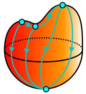
| The gradient trajectories on the sphere $S^2$ after creation of an index $1$ and $2$ cancelling pair of critical points. |
If we include the signs we have ignored, then $d_2 = \begin{pmatrix}1,1\end{pmatrix}$ and $d_1 = 0$ (because the two trajectories from the critical point of index $1$ to the critical point of index $0$ come with opposite sign, or alternatively, this is the only way to have $d^2 = 0$). We obtain the same Morse homology as before.
Remark: There's a bit of a technicality to this story, which is that we should really be working over $\mathbb{R}$ instead of $\mathbb{Z}$, since Witten's work does not actually reproduce the integral version. So everywhere we simply tensor our complex with $\mathbb{R}$. And actually, a critical point $p$ in the Morse-Smale-Witten complex should instead be thought of as $e^{tf(p)}p'$, for a different set of generators $p'$, where $t$ is a formal parameter. Then the numbers in the differential should be $e^{-t(f(p)-f(q))} \cdot n(p,q)$ instead of just $n(p,q)$. If you're familiar with Floer theory, this should look familiar, in the form of Novikov parameters.

Comments
Post a Comment